Interpolation in pure python

Posted on 23 February 2013

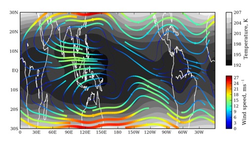
A long while ago, I wrote a script for matplotlib that later (after lots of work by Tony Yu and others) became the matplotlib streamplot function. This function generates plots that are constructed out of streamlines of a flow, in such a way as to fill the domain uniformly with such streamlines. I wrote the script to plot winds in the tropical upper troposphere/lower stratosphere where there is a lot of divergence and convergence (principally caused by convection over the western Pacific and subsidence over the eastern Pacific.)

The streamplot algorithm uses an adaptive 1st/2nd order Runge-Kutta scheme and linear interpolation of the velocity field to integrate the streamlines. This was implemented in pure python, which I originally chose to do because the portion of the algorithm responsible for ensuring an even domain-filling distribution of streamlines imposes a very strange termination condition on the integral that does not fit well with the integrators in scipy. In addition, matplotlib does not depend on scipy.

I initially expected a pure python algorithm to be incredibly slow, so I used a very simple interpolation scheme. Any interpolation scheme interpolating some data D[i] defined at points x[i] on to the target point x0 is composed of two steps; first, the algorithm must identify the nearest grid points to the target point. Second, the interpolator must apply the appropriate interpolator to those neighbouring points.

The second step is usually trivial to implement, but the first step is non-trivial in general. The first step becomes a lot simpler when we restrict ourselves to a regular grid with spacing dx as we can then find the index i of the point just above x0 by rescaling and casting to an integer

i = int(1 + (x0 - x[0]) / dx)

I thought this was probably the fastest way of implementing an interpolator and so used this technique to implement the interpolator in streamplot. However, it added some complexity to the algorithm and, most importantly, imposed a restriction that only regular grids (i.e. grids with evenly spaced axes) could be used. For my original purpose, this was not a problem but it is clearly a rather serious limitation in general.

Recently I have been hitting this limitation and decided over the last couple of evenings to try to free streamplot of this limitation. To generalise the first interpolation step to work with any x[i], a search is needed to find the smallest i such that x[i] > x0. Any pure python search algorithm would be too slow. Using argmax to do a linear search is an option:

i = numpy.argmax(x[i] > x0)

However, this does not scale well with the length of each dimension and is too slow in this context.

Looking through the standard library, I came across the bisect module which implements the interval bisection method for searching ordered lists and arrays – exactly what I needed to do. Implementing this search is really simple; it’s just

i = bisect.bisect(x, x0)

This method is really fast – way faster than I expected. After re-implementing the streamplot integrator and interpolator to use this type of interpolation, typical plotting times were barely increased.

Here is an example of the new script in action with a very non-uniform vertical grid spacing:

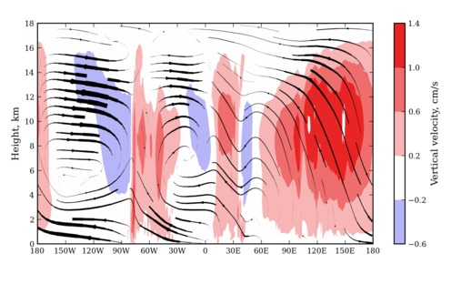
(This plot shows the boreal winter average zonal and vertical winds in the inner tropics.)

The new script is available here. Feel free to try it out if you need to do streamplots with uneven grids. Please note that this is a work-in-progress and so use with caution :-)